Neural Networks: Zero to Hero (Part 1)

This post contains my notes on the first video in Andrej Karpathy’s course: Neural Networks: Zero to Hero.

This Course

A course by Andrej Karpathy on building neural networks, from scratch, in code.

We start with the basics of backpropagation and build up to modern deep neural networks, like GPT. In my opinion language models are an excellent place to learn deep learning, even if your intention is to eventually go to other areas like computer vision because most of what you learn will be immediately transferable. This is why we dive into and focus on language models.

Prerequisites: solid programming (Python), intro-level math (e.g. derivative, gaussian).

I used Google Colab to setup the Python notebook; all source code can be found at this GitHub repo.

Micrograd

The video essential involves building micrograd from scratch, which is a tiny, efficient Autograd engine developed by Karpathy that uses very simple scalar values to implement backpropagation and a small neural networks library (with a PyTorch-like API). As the video progresses, we will be able to understand micrograd more and more.

This is a code snippet from micrograd’s GitHub readme:

from micrograd.engine import Value
 
a = Value(-4.0)
b = Value(2.0)
c = a + b
d = a * b + b**3
c += c + 1
c += 1 + c + (-a)
d += d * 2 + (b + a).relu()
d += 3 * d + (b - a).relu()
e = c - d
f = e**2
g = f / 2.0
g += 10.0 / f
print(f'{g.data:.4f}') # prints 24.7041, the outcome of this forward pass
g.backward()
print(f'{a.grad:.4f}') # prints 138.8338, i.e. the numerical value of dg/da
print(f'{b.grad:.4f}') # prints 645.5773, i.e. the numerical value of dg/db

Essentially, some scalar values are being initialized (a and b), and they are manipulated through addition, multiplication, and negation, exponential functions, and even squeezed to zero (.relu() basically returns the max of 0 and the input, zeroing out any negative values). The important line is when g.backward() is called, which initializes backprop at g, going backwards in the expression graph and recursively applying the chain rule of calculus which allows us to evaluate the partial differentiation of input variables.

This can be seen when a.grad is printed, which tells us how the function of g responds when a is increased by an infinitesimally small amount, which is basically the instantaneous slope or derivative $\frac{dg}{da}$, as it is known in the field of calculus.

Chain Rule

$\frac{dy}{dx}=\frac{dy}{du}\cdot \frac{du}{dx}$
For example, if $y=3(2x+2{)}^2$, $\frac{dy}{dx}=6u\cdot 2$, where $u=2x+2$. Chain rule involves taking the derivative of the outside, then multiplying by the derivative of the inside..

Explanation of Derivatives in Python

To start, all the basic libraries such as math, NumPy, and Matplotlib are imported.

import math
import numpy as np
import matplotlib.pyplot as plt
 
# Optional stylistic changes
import seaborn as sns
 
sns.set_theme(style="whitegrid", palette="muted")
plt.rcParams['figure.figsize'] = (10, 6)
plt.rcParams['figure.dpi'] = 100

Karpathy starts off by defining a function $f(x)=3x^2-4x+5$.

def f(x):
    return 3*x**2 - 4*x + 5

Calling f(3.0) passes in $3.0$ as the $x$ value into $f(x)$; this returns $20.0$.

We can apply this function $f(x)$ to a range of values using the arange() function from numpy.

xs = np.arange(-5, 5, 0.25) # this creates a range from -5 to 5, with steps of 0.25
xs

This outputs the numpy array xs: [-5.00, -4.75, -4.50, -4.25, -4.00, -3.75, -3.50, -3.25, -3.00, -2.75, -2.50, -2.25, -2.00, -1.75, -1.50, -1.25, -1.00, -0.75, -0.50, -0.25, 0.00, 0.25, 0.50, 0.75, 1.00, 1.25, 1.50, 1.75, 2.00, 2.25, 2.50, 2.75, 3.00, 3.25, 3.50, 3.75, 4.00, 4.25, 4.50, 4.75]
These values represent the y-values where $y=f(x)$. We can use matplotlib.pyplot to plot these values on a graph, plt.plot(xs, ys):

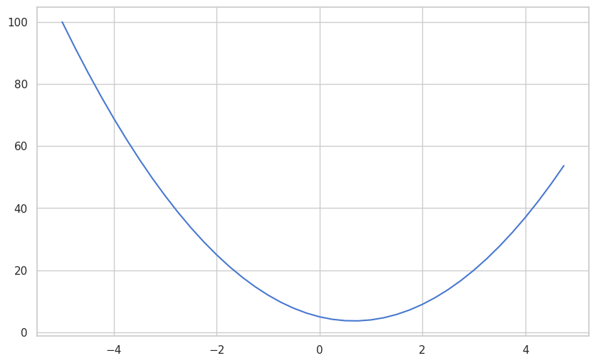
As expected, it is a parabola.

Now, if we derive the function $f(x)=3x^2-4x+5$ by hand, we can use power rule to get $f^{\prime }(x)=6x-4$.

Power Rule

$\frac{d}{dx}(x^n)=n{x}^{n-1}$

Plotting the derivative $f^{\prime }(x)=6x-4$ gives us a straight line:

# deriv of f(x) = f'(x) = 6x - 4
plt.plot(xs, 6 * xs - 4)

This makes sense because the derivative of a quadratic function is linear. The graph represents the instantaneous slope of the parabola $f(x)$ at every value of $x$.

• When the derivative is positive, the function is increasing.
• When the derivative is negative, the function is decreasing.
• When the derivative is 0, the function is not changing at that point, meaning it is possibly a local max or min.
  • For example, in this case, the slope/derivative of $f(x)$ is 0 when $x=\frac{2}{3}$. This is where the parabola has its minimum value.

Numerical Approximation of Derivatives

Solving the derivative by hand is trivial, until we have to solve it for actual machine learning models or even language models that can potentially use millions and billions of parameters (also known as weights, which are the coefficients of the inputs in a function). This is done by backprop, which will be explained in detail later, so for now we can attempt to approximate the derivative using the limit definition of a derivative:
$f^{\prime }(x)={\lim }_{h\to 0}\frac{f(x+h)-f(x)}{h}$
This looks familiar, as it is very similar to the slope formula between two points, which subtracts the y-values of the 2 points (this represents the rise), and divides by the difference in x-value (this represents the run): rise / run. In a similar fashion, to get the instantaneous slope at one point, we can add a very tiny number $h$ to the x-value to get our “second point”. This value $h$ approaches 0 so we can get as close to the true instantaneous slope as possible.

• $h$ is a very tiny number
• $f(x+h)-f(x)$ measures how much the function changes
• dividing by $h$ gives the rate of change

We can set this up in our Python notebook:

h = 0.001
x = 3.0

# limit definition of derivative
deriv = ( f(x + h) - f(x) ) / h
deriv

This computes $\frac{f(x+h)-f(x)}{h}$ and outputs this floating point number: 14.00300000000243, estimating the slope of the function at $x=3$.

At $x=3$:

$$f^{\prime }(x)=6x-4$$

so:

$$f^{\prime }(3)=14$$

The numerical approximation should therefore produce a value very close to $14$.

Differentiation with Multiple Inputs

Karpathy then switches to a much smaller expression graph:

a = 2.0
b = -3.0
c = 10
d = a*b + c
d

This evaluates to:

$$d=(2)(-3)+10=4$$

Now, we have multiple input variables $a$, $b$, and $c$, not just one variable $x$. The goal now is to understand how changing each input variable slightly affects the output $d$, also known as partial differentiation.

We can again use the limit definition of a derivative:

h = 0.0001
def d(a, b, c):
	return a*b + c
	
d1 = d(a, b, c)
d2 = d(a+h, b, c)
 
print("d1:", d1)
print("d2:", d2)
print("slope:", (d2 - d1) / h)

Only $a$ is changed slightly by adding $h$, and the output is -3.000000000010772.

Taking the partial derivative of $d=ab+c$ with respect to $a$:

$$\frac{\partial d}{\partial a}=b$$

And since $b=-3$:

$$\frac{\partial d}{\partial a}=-3$$

Therefore, the slope estimated by the code should be very close to $-3$.

We can do the same slight adjustment of $h$ to either $a$, $b$, or $c$, and get their respective partial derivatives. The closer $h$ gets to 0, the more accurate the estimation will be. However, Python has limited memory space for floating point numbers, so eventually it will not work as intended.

This is the core intuition behind these partial derivatives or gradients:

A derivative tells us how sensitive the output is to a specific input variable.

In neural networks, these gradients allow us to determine how much to change weights and biases by, and how that affects the loss function (a decrease in loss would be an improvement in the neural network).

Creating a Value Object

Karpathy then begins to build the foundations of his library micrograd by creating a custom Value class.

class Value:
	def __init__(self, data, _children=(), _op=''):
	    self.data = data
	    self._children = set(_children)
	    self._op = _op_
 
    def __repr__(self):
        return f"Value(data={self.data})"
 
    def __add__(self, other):
        return Value(self.data + other.data, (self, other), '+')
 
    def __mul__(self, other):
        return Value(self.data * other.data, (self, other), '*')

__init__

def __init__(self, data, _children=(), _op=''):
    self.data = data
    self._children = set(_children)
    self._op = _op_

The constructor stores the scalar value inside the object.

__repr__

def __repr__(self):
    return f"Value(data={self.data})"

This controls how the object is displayed when printed.

Without this method, Python would show something like:

<__main__.Value object at 0x000001...>

Instead, we now get readable outputs like:

Value(data=2.0)

Operator Overloading

Karpathy also overloads mathematical operators such as + and *.

def __add__(self, other):
    return Value(self.data + other.data, (self, other), '+')
 
def __mul__(self, other):
    return Value(self.data * other.data, (self, other), '*')

This allows us to manipulate Value objects just like numbers.

Using the Value Class

a = Value(2.0)
b = Value(-3.0)
c = Value(10.0)
a, b, c

Output:

(Value(data=2.0), Value(data=-3.0), Value(data=10.0))

Addition now works:

a + b

which returns:

Value(data=-1.0)

Multiplication also works:

a * b

which returns:

Value(data=-6.0)

And entire expressions can now be constructed:

a*b + c

which evaluates to:

Value(data=4.0)

At this point, these objects only store data and basic operations. However, the next step in micrograd is much more important:

• storing how values were created,
• constructing a computational graph,
• and eventually implementing automatic backpropagation through that graph.